
主成分分析
1.概要
主成分分析法由Karl Pearson 在 1903 提出,经由Harold Hotelling 在 20世纪三十年代从另一个角度进行了完善,是一种适用于高维数据,探索性数据分析的方法,作为最早一批被应用于模式识别、机器学习模型的算法之一,其现在经过实现数据压缩降维、特征提取而广泛应用于力学、信号处理、质量控制、心理学等许多领域。
2.算法思想
简单一句话来说的话:找到一组组正交化的投影(一次线性变化-linear transformation),使得原空间的数据在新的投影空间中的数据方差最大,也即尽可能使投影结果分散。而如何去找到这样的一个线性变化呢? 这时候不得不说数学家们的想法是真的难以想象。
假设有这样一组n个样本的数据,每个样本有d个特征X ={ },我们对数据样本进行中心化(Data centralisation)
其中m为所有样本的中心。
接着为了找到第一主成分的投影 u 使得该投影空间下数据的方差最大,
令,则样本空间的方差D可以表示为:
此处m为新样本的中心,由于原数据进行了中心化,易得:
则
其中不难发现为原空间数据X的斜方差矩阵,这里使得投影向量的长度
.问题变转化成了求函数:
求最值问题。 接着借助拉格朗日乘子法我们可以将上述函数转化成如下形式:
,
对u求偏导易得:
2Su − 2λu = 0 也即Su= λu
这时我们可以看出u和λ即为矩阵S一一对应的特征向量和特征值。
所以求解最大化D也就是求得最大的特征值λ,最大特征值对应的特征向量便是我们要求的“第一主成分” 。 利用同样的方法,易知矩阵S协方差矩阵的特征值从大到小排列其对应的前P个特征向量即为所求线性变换的转换矩阵。
def pca(X):
n_points, n_features = X.T.shape #to get the number of samples and the number features of each sample
mean = np.array([np.mean(X.T[:,i]) for i in range(n_features)]) #to get the mean matrix of feachures
#Centralization
cen_X = X.T-mean
#empirical covariance matrix
cov_matrix = np.dot(cen_X.T,cen_X)/(n_points-1)
#then to calculate the eigenvectors and eigenvalues using np.linalg.eig, in the numpy
eig_val, eig_vec = np.linalg.eig(cov_matrix)
res = {}
for i in range(len(eig_val)):
res[eig_val[i]] = eig_vec[i]
return eig_val, eig_vec
# Visualisation
val, vec = my_pca(X)
X=X.T
dic = {}
for i in range(len(val)):
dic[val[i]] = vec[i]
ls = sorted(dic,reverse=True)
k = 2 # to select the first 2 principal components(pc1 pc2)
new_features = np.array([dic[e] for e in ls[:k]])
print(new_features)
n_points, n_features = X.shape
mean = np.array([np.mean(X[:,i]) for i in range(n_features)])
cen_X = X-mean
print(cen_X.shape)
data=np.dot(cen_X,np.transpose(new_features))
x=[]
y = []
x.append(data.T[0])
y.append(data.T[1])
# to select the first and the third principal components(pc1 pc3)
new_features_13 = np.array([dic[ls[0]],dic[ls[2]]])
data_13=np.dot(cen_X,np.transpose(new_features_13))
x.append(data_13.T[0])
y.append(data_13.T[1])
# to select the second and the third principal components(pc2 pc3)
new_features_23 = np.array([dic[ls[1]],dic[ls[2]]])
data_23=np.dot(cen_X,np.transpose(new_features_23))
x.append(data_23.T[0])
y.append(data_23.T[1])
# to show the data sets after PCA and being projected to 2D
for i in range(len(x)):
plt.scatter(x[i],y[i])
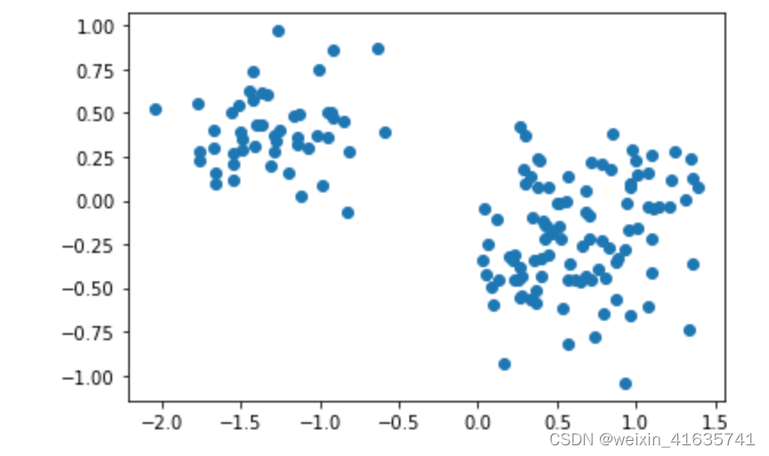
plt.show()分别选择不同的主成分构造线性变换的矩阵进行投影:
选择所对应的向量进行压缩变换:
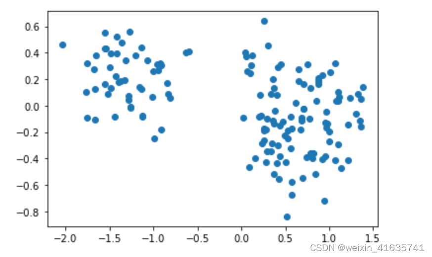
选择所对应的向量进行压缩变换:
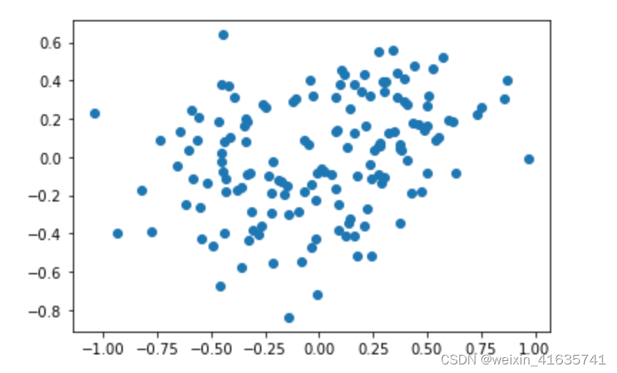
选择所对应的向量进行压缩变换:
(明天补充Dual PCA)