
【optimtool】1.1.3版本使用文档
版权归属:林景 (MIT Lisence)
pip install optimtool
1. 无约束优化算法性能对比
import sympy as sp
import matplotlib.pyplot as plt
from optimtool.unconstrained import gradient_descent, newton, newton_quasi, trust_region

f, x1, x2, x3, x4 = sp.symbols("f x1 x2 x3 x4")
f = (x1 - 1)**2 + (x2 - 1)**2 + (x3 - 1)**2 + (x1**2 + x2**2 + x3**2 + x4**2 - 0.25)**2
funcs = sp.Matrix([f])
args = sp.Matrix([x1, x2, x3, x4])
x_0 = (1, 2, 3, 4)

# 无约束优化测试函数性能对比
f_list = []
title = ["gradient_descent_barzilar_borwein", "newton_CG", "newton_quasi_L_BFGS", "trust_region_steihaug_CG"]
colorlist = ["maroon", "teal", "slateblue", "orange"]
_, _, f = gradient_descent.barzilar_borwein(funcs, args, x_0, False, True)
f_list.append(f)
_, _, f = newton.CG(funcs, args, x_0, False, True)
f_list.append(f)
_, _, f = newton_quasi.L_BFGS(funcs, args, x_0, False, True)
f_list.append(f)
_, _, f = trust_region.steihaug_CG(funcs, args, x_0, False, True)
f_list.append(f)

# 绘图
handle = []
for j, z in zip(colorlist, f_list):
    ln, = plt.plot([i for i in range(len(z))], z, c=j, marker='o', linestyle='dashed')
    handle.append(ln)
plt.xlabel("$Iteration \ times \ (k)$")
plt.ylabel("$Objective \ function \ value: \ f(x_k)$")
plt.legend(handle, title)
plt.title("Performance Comparison")
plt.show()
图像:

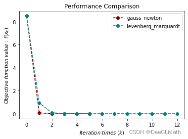
2. 非线性最小二乘问题
import sympy as sp
import matplotlib.pyplot as plt
from optimtool.unconstrained import nonlinear_least_square

r1, r2, x1, x2 = sp.symbols("r1 r2 x1 x2")
r1 = x1**3 - 2*x2**2 - 1
r2 = 2*x1 + x2 - 2
funcr = sp.Matrix([r1, r2])
args = sp.Matrix([x1, x2])
x_0 = (2, 2)

f_list = []
title = ["gauss_newton", "levenberg_marquardt"]
colorlist = ["maroon", "teal"]
_, _, f = nonlinear_least_square.gauss_newton(funcr, args, x_0, False, True) # 第五参数控制输出函数迭代值列表
f_list.append(f)
_, _, f = nonlinear_least_square.levenberg_marquardt(funcr, args, x_0, False, True)
f_list.append(f)

# 绘图
handle = []
for j, z in zip(colorlist, f_list):
    ln, = plt.plot([i for i in range(len(z))], z, c=j, marker='o', linestyle='dashed')
    handle.append(ln)
plt.xlabel("$Iteration \ times \ (k)$")
plt.ylabel("$Objective \ function \ value: \ f(x_k)$")
plt.legend(handle, title)
plt.title("Performance Comparison")
plt.show()
图示:
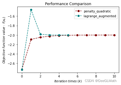
3. 等式约束优化测试
import numpy as np
import sympy as sp
import matplotlib.pyplot as plt
from optimtool.constrained import equal

f, x1, x2 = sp.symbols("f x1 x2")
f = x1 + np.sqrt(3) * x2
c1 = x1**2 + x2**2 - 1
funcs = sp.Matrix([f])
cons = sp.Matrix([c1])
args = sp.Matrix([x1, x2])
x_0 = (-1, -1)

f_list = []
title = ["penalty_quadratic", "lagrange_augmented"]
colorlist = ["maroon", "teal"]
_, _, f = equal.penalty_quadratic(funcs, args, cons, x_0, False, True) # 第四个参数控制单个算法不显示迭代图,第五参数控制输出函数迭代值列表
f_list.append(f)
_, _, f = equal.lagrange_augmented(funcs, args, cons, x_0, False, True)
f_list.append(f)

# 绘图
handle = []
for j, z in zip(colorlist, f_list):
    ln, = plt.plot([i for i in range(len(z))], z, c=j, marker='o', linestyle='dashed')
    handle.append(ln)
plt.xlabel("$Iteration \ times \ (k)$")
plt.ylabel("$Objective \ function \ value: \ f(x_k)$")
plt.legend(handle, title)
plt.title("Performance Comparison")
plt.show()
图示:
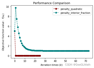
4. 不等式约束优化测试
import sympy as sp
import matplotlib.pyplot as plt
from optimtool.constrained import unequal

f, x1, x2 = sp.symbols("f x1 x2")
f = x1**2 + (x2 - 2)**2
c1 = 1 - x1
c2 = 2 - x2
funcs = sp.Matrix([f])
cons = sp.Matrix([c1, c2])
args = sp.Matrix([x1, x2])
x_0 = (2, 3)

f_list = []
title = ["penalty_quadratic", "penalty_interior_fraction"]
colorlist = ["maroon", "teal"]
_, _, f = unequal.penalty_quadratic(funcs, args, cons, x_0, False, True) # 第四个参数控制单个算法不显示迭代图,第五参数控制输出函数迭代值列表
f_list.append(f)
_, _, f = unequal.penalty_interior_fraction(funcs, args, cons, x_0, False, True)
f_list.append(f)

# 绘图
handle = []
for j, z in zip(colorlist, f_list):
    ln, = plt.plot([i for i in range(len(z))], z, c=j, marker='o', linestyle='dashed')
    handle.append(ln)
plt.xlabel("$Iteration \ times \ (k)$")
plt.ylabel("$Objective \ function \ value: \ f(x_k)$")
plt.legend(handle, title)
plt.title("Performance Comparison")
plt.show()
图示:
5. 混合等式约束测试
import sympy as sp
import matplotlib.pyplot as plt
from optimtool.constrained import mixequal

f, x1, x2 = sp.symbols("f x1 x2")
f = (x1 - 2)**2 + (x2 - 1)**2
c1 = x1 - 2*x2
c2 = 0.25*x1**2 - x2**2 - 1
funcs = sp.Matrix([f])
cons_equal = sp.Matrix([c1])
cons_unequal = sp.Matrix([c2])
args = sp.Matrix([x1, x2])
x_0 = (0.5, 1)

# 无约束优化测试函数性能对比
f_list = []
title = ["penalty_quadratic", "penalty_L1", "lagrange_augmented"]
colorlist = ["maroon", "teal", "orange"]
_, _, f = mixequal.penalty_quadratic(funcs, args, cons_equal, cons_unequal, x_0, False, True) # 第四个参数控制单个算法不显示迭代图,第五参数控制输出函数迭代值列表
f_list.append(f)
_, _, f = mixequal.penalty_L1(funcs, args, cons_equal, cons_unequal, x_0, False, True)
f_list.append(f)
_, _, f = mixequal.lagrange_augmented(funcs, args, cons_equal, cons_unequal, x_0, False, True)
f_list.append(f)

# 绘图
handle = []
for j, z in zip(colorlist, f_list):
    ln, = plt.plot([i for i in range(len(z))], z, c=j, marker='o', linestyle='dashed')
    handle.append(ln)
plt.xlabel("$Iteration \ times \ (k)$")
plt.ylabel("$Objective \ function \ value: \ f(x_k)$")
plt.legend(handle, title)
plt.title("Performance Comparison")
plt.show()
图示:

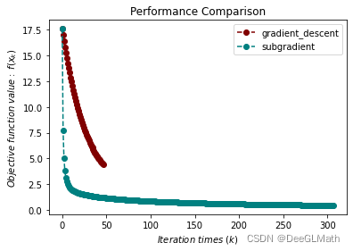
6. Lasso问题测试
min
1
2
∣
∣
A
x
−
b
∣
∣
2
+
μ
∣
∣
x
∣
∣
1
\min \frac{1}{2} ||Ax-b||^2+\mu ||x||_1
min21∣∣Ax−b∣∣2+μ∣∣x∣∣1
给定
A
m
×
n
A_{m \times n}
Am×n,
x
n
×
1
x_{n \times 1}
xn×1,
b
m
×
1
b_{m \times 1}
bm×1,正则化常数
μ
\mu
μ。解决该无约束最优化问题,该问题目标函数一阶不可导。
import numpy as np
import sympy as sp
import matplotlib.pyplot as plt
from optimtool.unconstrained import Lasso

import scipy.sparse as ss
f, A, b, mu = sp.symbols("f A b mu")
x = sp.symbols('x1:9')
m = 4
n = 8
u = (ss.rand(n, 1, 0.1)).toarray()
A = np.random.randn(m, n)
b = A.dot(u)
mu = 1e-2
args = sp.Matrix(x)
x_0 = tuple([1 for i in range(8)])

# 无约束优化测试函数性能对比
f_list = []
title = ["gradient_descent", "subgradient"]
colorlist = ["maroon", "teal"]
_, _, f = Lasso.gradient_decent(A, b, mu, args, x_0, False, True)# 第四个参数控制单个算法不显示迭代图,第五参数控制输出函数迭代值列表
f_list.append(f)
_, _, f = Lasso.subgradient(A, b, mu, args, x_0, False, True)
f_list.append(f)

# 绘图
handle = []
for j, z in zip(colorlist, f_list):
    ln, = plt.plot([i for i in range(len(z))], z, c=j, marker='o', linestyle='dashed')
    handle.append(ln)
plt.xlabel("$Iteration \ times \ (k)$")
plt.ylabel("$Objective \ function \ value: \ f(x_k)$")
plt.legend(handle, title)
plt.title("Performance Comparison")
plt.show()
图示:
7. 待解决
- hybrid板块
- 无约束与有约束的应用问题(逻辑回归,相位复原等)
- 内点法的迭代溢出问题